Does P50 in equal P50 out? The answer is, ‘very rarely!’

This article directly follows on from Article 14 and so I would recommend you read that article first. Now I’ve tried to explain slippage previously in Article 9, although in that article I used a very simple example for illustrative purposes. That was because I only had Mathematics at the time to call upon to help in arriving at solutions. But recently I’ve come across an awesome tool that allows scheduling to be carried out on a probabilistic basis, giving me the ability to carry out more comprehensive examples and therefore highlight critical concepts. I have been given permission by BHP to use this tool to demonstrate the concepts presented in this article. Please also refer to the reference (Bloss et al, 2020) presented in Article 14 to understand the concept of schedule time slippage and the basis of this probabilistic scheduling tool development.

So in this article, I want to highlight why P50 in does not equal P50 out and that in fact, the differential is so large, even I was shocked at the size of the gap. As I did in Article 9, I am still going to run with a fairly simple case with 6 sequential activities, so each activity must be finished before the following activity can be started. Those activities are:

1.      Drill

2.      Blast

3.      Excavate waste

4.      Excavate ore

5.      Process ore

6.      And rail the ore. 

In this example I have assumed the mine is a balanced system, that is the equipment is all sized so that it has the same annual capacity, which means there is no planned idle time stemming from excess capacity. This is typically representative of the mining industry, as one of the strongest drivers in our industry is to not have equipment idle, it must be working at all times.

Because the capacities are balanced, all tasks take the same time period. In this example I have assumed 12 days for each task. All tasks are normally distributed and have a standard deviation that is 30% of the task length, so 3.6 days.

In this example mine, there is only one of each equipment type, so it is fully sequential. The drill can’t start one block until it has finished another block, as there is only one drill on site. I’ve simulated the mine over a long enough period that continual operation exists, so all equipment have tasks to be completed throughout the entire schedule. A snapshot of a portion of the simulated schedule is as per Figure 1 below. 

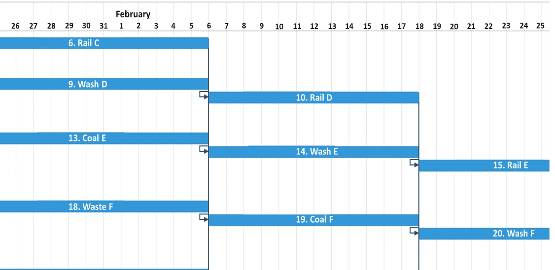
Figure 1 – Schedule Overview

As discussed in Article 14, slippage occurs when tasks have multiple dependencies. For example, Block B can’t be blasted until it has been drilled, but there is only one blast crew, which is not available until after they have blasted Block A. So, in this simple example, I have looked at a snapshot of the schedule starting on January 1st, when we commence railing Block A and have scheduled through to April. However, for comparison purposes, the date I am interested in is the date when Block F completes railing. In the deterministic schedule, there are 6 blocks of coal to be railed at a task length of 12 days each and with no gaps between those tasks, that is 72 days and so Block F completes railing on March 13th. 

Figure 2 displays the impacts once we introduce the variability of 3.6 days standard deviation for all of the tasks. The blue bars in the image portray the deterministic tasks and their planned start and end dates. The red bars display the 25th percentile, 50th percentile and 75th percentile completion dates following simulation of the schedule. Blasting Block E and Drilling Block F start on January 1; as the schedule only begins on January 1, these tasks are not dependent on any other tasks and therefore have a 50% probability of finishing on January 13. Blasting Block F, however, is dependent on the blast crew having blasted Block E and the drill having finished Block F and both activities could finish early or late.  But as discussed in Article 14, in 75% of the cases a delay will be passed through the system to the next task. Multiple dependencies lead to slippage, so the P50 completion date for blasting Block F has slipped 1.5 days to halfway through January 26. 

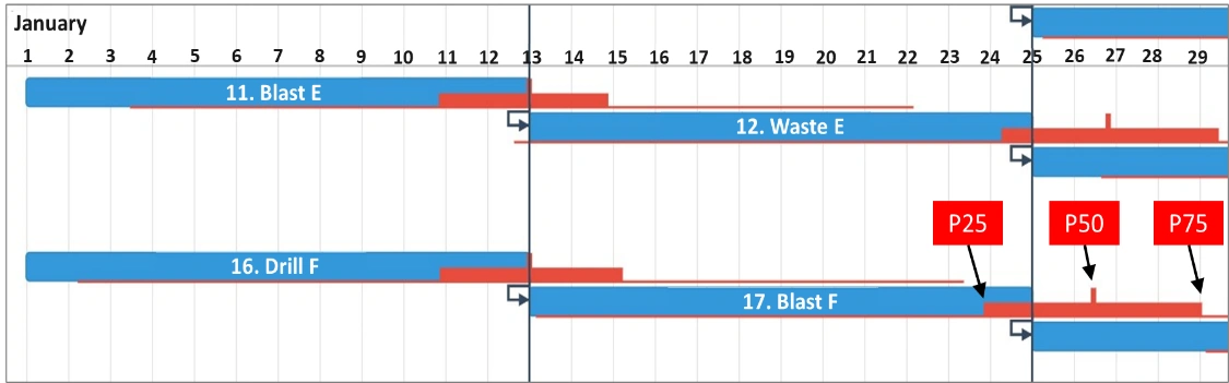
Figure 2 – Schedule Slippage

This slippage continues to grow throughout the schedule, highlighting that gains are lost, while losses accumulate throughout the system. Figure 3 shows the scheduling of all tasks for Block F from drilling through to railing. Sections A, B and C are sequential snapshots of the schedule (C follows B which follows A), but have been placed vertically below each other in this figure to fit in a portrait mode document. As shown, the slippage for the tasks are as follows:

· blast completion = 1.5 days; 

· waste excavation completion = 3.5 days;

· ore excavation completion = 6 days;

· washing completion = 8 days; and,

· railing completion = 10 days. 

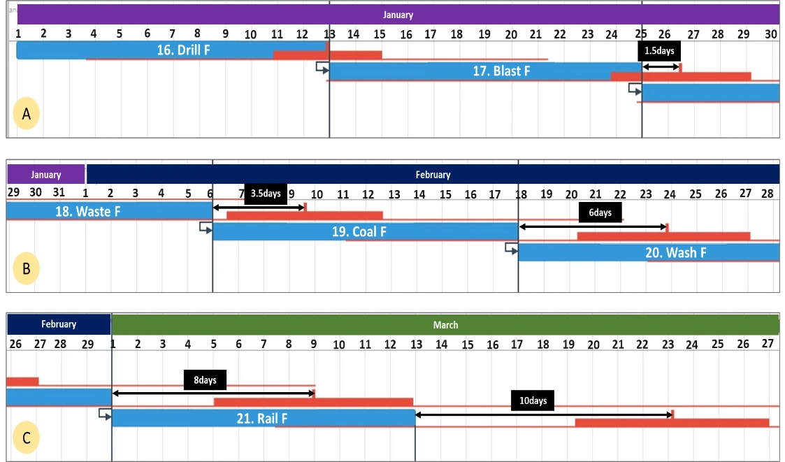
Figure 3 – Blast Slippage

Total slippage across the 72-day period of this schedule is 10 days, which equates to a 14% delay. There is also a 25% probability that the task won’t finish until March 27, a slippage of 14 days, or 19%. However, what I found quite remarkable, was the plan output probability, the probability of railing on time as per the deterministic schedule date of March 13 is only 2%, in other words a P02. 

So, in this example, P50 in definitely does not equal P50 out!

Alternatively, let’s say that mine management understands there is a difference between input probability and output probability so they actually want a mine plan that achieves P50 for the plan outputs. To achieve that in the above example would mean that the plan inputs required would have to have a 72% probability of being achieved in order to compensate for the time slippage. So P72 in, equals P50 out. Now, let’s understand what P72 inputs mean. It means that for a task that would take 10 days using mean input assumptions (deterministic), it is actually going to be scheduled to take 11.8 days (or 18% longer) to allow for the slippage that’s going to occur.  Now that sounds fine, until the production team and site management understand that you’re scheduling tasks to take 18% longer than target. That won’t sit well, as there will be a belief that the plan is driving the wrong behaviour in lowering productivity expectations. 

The above analysis highlights why we build inventory between tasks in mining operations, because it increases the probability that equipment can continue to operate and is not held up by the preceding activity in the sequence. Let’s run this same example but this time introduce inventories, allowing us to understand the impacts of inventory. Mine sites vary significantly in the inventories they hold and not all of that inventory is between tasks within the schedule. But, it is not uncommon for the blast crew to commence loading the shot as soon as it is finished drilling, or that the excavator starts digging the shot within a week of it being fired and ore is often mined as soon as the waste is removed. 

I’m going to introduce time buffers into the schedule as a representation of inventories and will run an example with five-day time buffers between all activities. This five-day buffer will only be created for the task dependencies, there will be no time buffers for the resource dependencies. As shown in Figure 4, the equipment will still operate on a continuous basis. For example, when the drill finishes drilling Block G, it goes straight to drill Block H, it doesn’t sit for any time idle between these tasks (resource buffer). However, when Block G is finished being drilled, there is a five-day buffer before Block G blasting commences. 

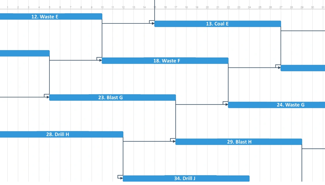
Figure 4 – Five Day Time Buffers

Figure 5 displays the time slippage that occurs now that time buffers have been introduced into the schedule. The time slippage for this schedule is now as follows:

· blast completion = 0.5 days; 

· waste excavation completion = 1 day;

· ore excavation completion = 2 days;

· washing completion = 3 days; and,

· railing completion = 4 days. 

Total slippage across the 72-day period of this schedule is 4 days, which equates to a 6% delay. In this example, the plan output probability has improved, the probability of railing on time, as per the deterministic schedule date of March 13, is now 29% (P29). 

So, in this example as well, P50 in definitely does not equal P50 out!

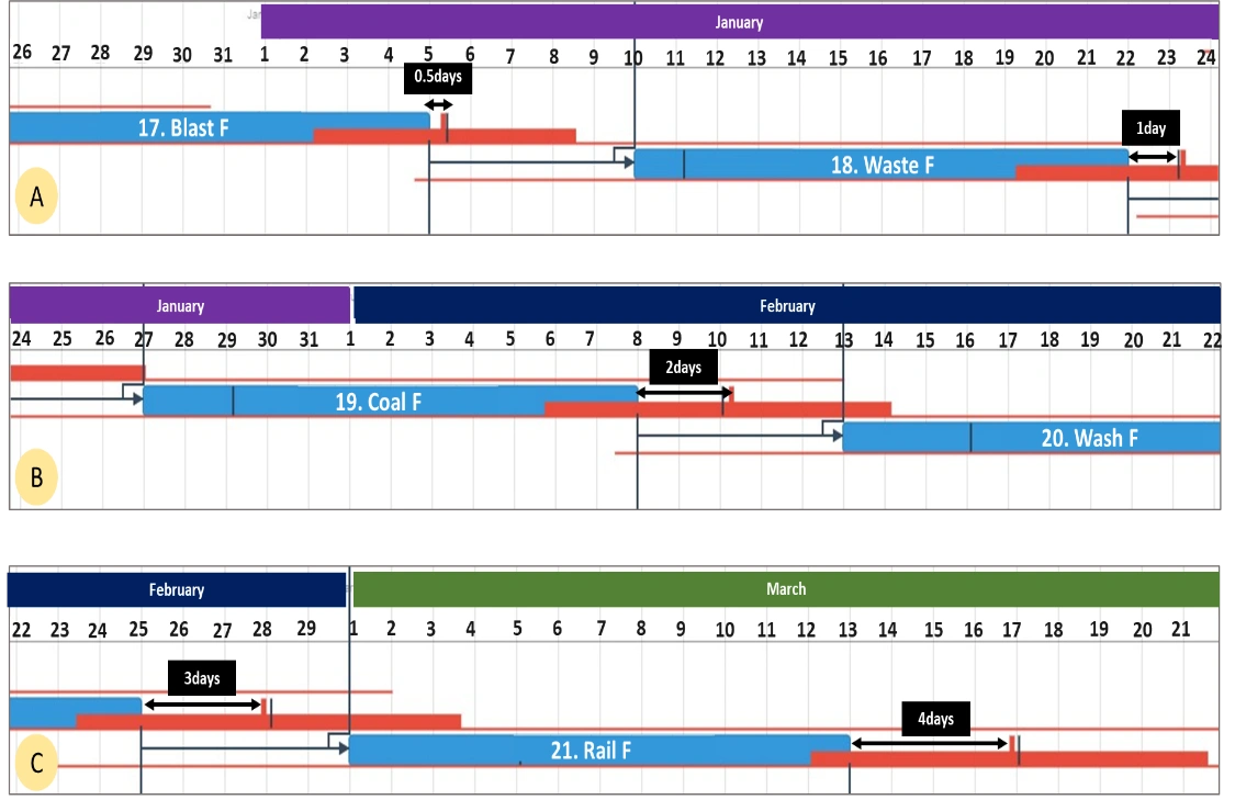
Figure 5 – Five Day Buffer Schedule Slippage

Next I found myself wondering, what is required for a P50 in plan to result in a P50 out plan? So I ran a number of variations of the above example and varied the time buffers, those results are shown in Table 1. The last row of this table is the input assumption probability required to achieve a 50% probability of achieving output assumptions. At buffer lengths of 13 days we still only have a P44 out plan and the minimal increase in P out between the 10 day and 13 day cases implies that buffers would have to be very, very large before P50 in equals P50 out in the plan  

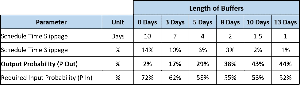
Table 1 – Simulation Results

It is interesting to note that, with the introduction of inventories, only a very minor shift in the input assumption probabilities is required to achieve a P50 out plan. For example, with buffer lengths of 8 days, P55 input assumptions will result in a P50 output plan. With the parameters used in this example, P55 input means you’re going to schedule the task at 3.5% below its expected (P50) production rate.

This example was built on activities that all had uniform task lengths of 12 days per task and with constant time buffers between every task. This is obviously an over-simplification of mine scheduling where task lengths vary substantially, as do time buffers between activities. However, at 13 days of time buffer, the buffers are actually greater in length than the actual task times (12 days) and we are still only at P44. So, I think it is safe to say that unless you are carrying massive inventories: 

P50 in DOES NOT equal P50 out!

What really strikes me after doing the work to write this chapter is how much we under-rate slippage in the mining industry and the degree to which we underestimate its impact. When I think back about it, schedule slippage is not a term that I’ve ever heard used when discussing schedules, it is not something that I have ever seen actually allowed for in any schedules and it is not a KPI measure that I’ve ever seen in any mine plans. I suspect this is largely because we (mining) have always lived in a deterministic world and we don’t have the scheduling software to easily identify, quantify and allow for slippage.

But what I really find incredulous is the lack of attention (that I’ve ever noticed anyway) to an issue that has such a large impact on throughput. If the mine is running with minimal inventories, then the ore railed is likely to be in the range of 5 – 15% less than planned. Let’s take an alternate scenario where all of the mine site equipment was operating at 10% below expected productivity leading to 10% less ore than planned, do you think that would be noticed? Do you think that would get some management attention, with significant efforts to solve it and a recovery plan put in place? Absolutely! 

However, we can have 10% slippage in our mine plans, plan after plan and it sits quietly under the radar. Why? I believe because we don’t understand it, we don’t measure it, and with the high frequency of changes to plan and other inherent mine planning issues, we’re not even aware that we are suffering 10% slippage in our mine plans. This is one of the significant benefits of probabilistic (or stochastic) scheduling, they are based on a deterministic schedule as the underlying plan. So any slippage is immediately evident, can be measured and we can start to bring this issue to light.

Here is my closing question for you, please leave some feedback via a comment on the post, it will be very helpful for future articles. “What question or questions does this article lead you to next?” For me, the first thing it leads to is “where is the best place for inventory (in a balanced system)?” But someone else has said to me “what does it look like if it is a skewed distribution rather than normal?” Let me know your questions.

This article is the fifteenth in a series of articles on various issues and topics relating to mine scheduling. If you found this article beneficial, you can always go back to the first article here and read through the series in order.

For other articles like this and quality conversations on a range of mining engineering subjects, I’d encourage you to join the LinkedIn Group called MinErs Digs, click here.